Exercises

1. Submission
2. 👤 Individual
   1. 📨 Deliverable 1 - Single-segment trajectory optimization (20 pts)
   2. 📨 Deliverable 2 - Multi-segment trajectory optimization (15 pts)
3. 👥 Team
   1. 📨 Deliverable 3 - Drone Racing (65 pts)
      1. Graded GitHub files checklist
      2. Setting up your codebase
      3. Coding – Part 0
      4. Coding – Parts 1.1, 1.2, and 1.3
      5. Recording a Video and ROS2 Bag
      6. Submitting your code
      7. [Optional] Faster, faster (Extra credit: 15 pts)
      8. [Optional] Provide feedback (Extra credit: 3 pts)

Submission

To submit your assignment, please do the following:

• Submit the individual math-related tasks as a typeset PDF to GradeScope.
• Submit the team’s coding-related tasks to your team-submissions repository (instructions below).

Deadline: the VNAV staff will clone your repository on October 2nd at 1 PM ET.

👤 Individual

📨 Deliverable 1 - Single-segment trajectory optimization (20 pts)

Consider the following minimum velocity ($r=1$) single-segment trajectory optimization problem:

with $P(t) \in \mathbb{R}[t]$, i.e., $P(t)$ is a polynomial function in $t$ with real coefficients:

\begin{equation} P(t) = p_N t^N + p_{N-1} t^{N-1} + \dots + p_1 t + p_0. \end{equation}

Note that because of constraint (\ref{eq:initpos}), we have $P(0)=p_0=0$, and we can parametrize $P(t)$ without a scalar part $p_0$.

1. Suppose we restrict $P(t) = p_1 t$ to be a polynomial of degree 1, what is the optimal solution of problem (\ref{eq:minvel})? What is the value of the cost function at the optimal solution?

2. Suppose now we allow $P(t)$ to have degree 2, i.e., $P(t) = p_2t^2 + p_1 t$.

(a) Write $\int_0^1 (P^{(1)}(t))^2 dt$, the cost function of problem (\ref{eq:minvel}), as $\boldsymbol{p}^T \boldsymbol{Q} \boldsymbol{p}$, where $\boldsymbol{p} = [p_1,p_2]^T$ and $\boldsymbol{Q} \in \mathcal{S}^2$ is a symmetric $2\times 2$ matrix.

(b) Write $P(1) = 1$, constraint (\ref{eq:finalpos}), as $\boldsymbol{A}\boldsymbol{p} = \boldsymbol{b}$, where $\boldsymbol{A} \in \mathbb{R}^{1 \times 2}$ and $\boldsymbol{b} \in \mathbb{R}$.

(c) Solve the Quadratic Program (QP): \begin{equation} \min_{\boldsymbol{p}} \boldsymbol{p}^T \boldsymbol{Q} \boldsymbol{p} \quad s.t. \quad \boldsymbol{A} \boldsymbol{p} = \boldsymbol{b}. \label{eq:QPtrajOpt} \end{equation} You can solve it by hand, or you can solve it using numerical QP solvers (e.g., you can easily use the quadprog function in Matlab). What is the optimal solution you get for $P(t)$, and what is the value of the cost function at the optimal solution? Are you able to get a lower cost by allowing $P(t)$ to have degree 2?

3. Now suppose we allow $P(t) = p_3t^3 + p_2 t^2 + p_1 t$:

(a) Let $\boldsymbol{p} = [p_1,p_2,p_3]^T$, write down $\boldsymbol{Q} \in \mathcal{S}^3, \boldsymbol{A} \in \mathbb{R}^{1\times 3}, \boldsymbol{b} \in \mathbb{R}$ for the QP (\ref{eq:QPtrajOpt}).

(b) Solve the QP, what optimal solution do you get? Do this example agree with the result we learned from Euler-Lagrange equation in class?

4. Now suppose we are interested in adding one more constraint to problem (\ref{eq:minvel}):

\begin{eqnarray} \min_{P(t)} \quad \int_0^1 (P^{(1)}(t))^2 dt, \label{eq:minveladd} \
s.t. \quad P(0) = 0, \
\quad P(1) = 1, \
\quad P^{(1)}(1) = -2. \end{eqnarray} Using the QP method above, find the optimal solution and optimal cost of problem (\ref{eq:minveladd}) in the case of:

(a) $P(t) = p_2t^2 + p_1 t$, and

(b) $P(t) = p_3t^3 + p_2 t^2 + p_1t$.

📨 Deliverable 2 - Multi-segment trajectory optimization (15 pts)

1. Assume our goal is to compute the minimum snap trajectory ($r= 4$) over $k$ segments. How many and which type of constraints (at the intermediate points and at the start and end of the trajectory) do we need in order to solve this problem? Specify the number of waypoint constraints, free derivative constraints and fixed derivative constraints.

• Hint: According to Euler-Lagrange method, what is the degree of the polynomial of each segment?
• Hint: How many unknown parameters do we need to solve?
• Hint: How many constraints does each waypoint/free derivative/fixed derivative constraint provide?
• Hint: See figure for $k=3$ as described in the lecture notes.

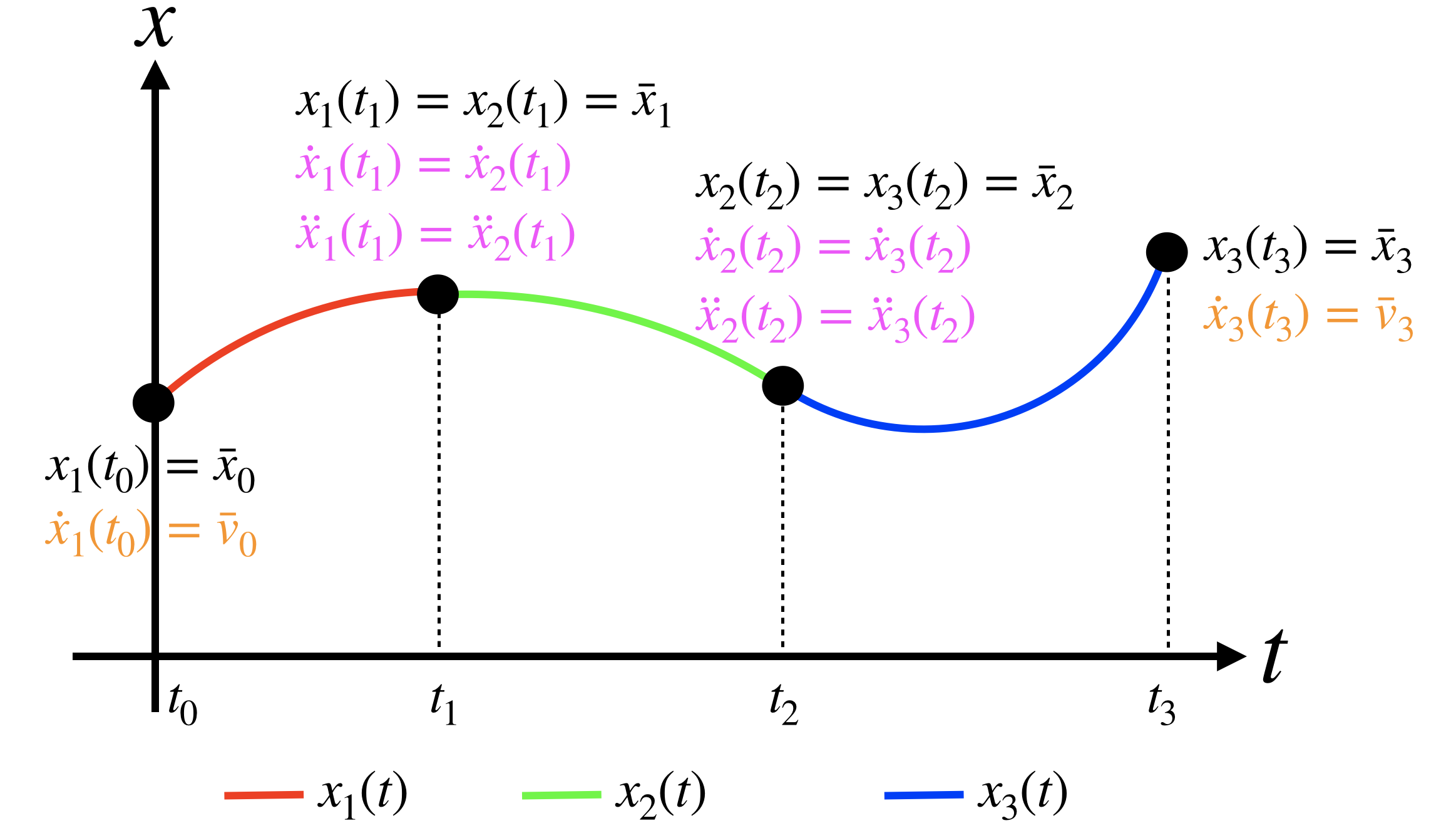
2. Can you extend the previous question to the case in which the cost functional minimizes the $r$-th derivative and we have $k$ segments?

👥 Team

📨 Deliverable 3 - Drone Racing (65 pts)

For this lab we will be racing our simulated our simulated quadcopters in a drone racing course we prepared in our Unity simulator!

Graded GitHub files checklist

• Implement all the missing parts in the code:
  • Part 0 → planner_pkg/src/simple_traj_planner.cpp
  • Part 1.1 → trajectory_generation_pkg/src/trajectory_generation_node.cpp
  • Part 1.2 → trajectory_generation_pkg/src/trajectory_generation_node.cpp
  • Part 1.3 → trajectory_generation_pkg/src/trajectory_generation_node.cpp
• Create a file called links.txt with two publically links (i.e., hosted on either Google Drive or Dropbox) to the following deliverables:
  • A video (i.e., ideally a screen capture) showing your quadrotor completing the race course.
  • A ROS2 bag recording of your complete and fastest run. In ROS2 this a bag recording is a folder with a metadata.yaml and .db3 file(s) – i.e., it is no longer a single .bag files as in ROS1. Instructions on how to record are below.

Setting up your codebase

Moving forward, we will be using the following file structure:

~/vnav
├── starter-code → cloned from https://github.com/MIT-SPARK/VNAV-labs
│   ├── ...  → starter code for previous labs
│   └── lab4 → start code for this lab
├── team-submissions → cloned from https://github.mit.edu/VNAV2024-submissions
│   ├── ...  → simulator files for previous labs
│   └── lab4 → this lab's graded code files need to be commited/pushed here
├── personal-submissions → cloned from https://github.mit.edu/VNAV2024-submissions
│   └── ...  → submission code from previous labs (no personal code for lab4)
├── tesse → create this folder for downloading/unzipping simulator code
│   ├── lab3 → download/unzip from https://vnav.mit.edu/material/lab3.zip
│   └── lab4 → download/unzip from https://vnav.mit.edu/material/lab4.zip
└── ws → `colcon` workspaces for each assignment
    ├── ...  → ros2 workspaces for previous labs
    └── lab4 → ros2 workspace for lab4
        ├── build   → generated by `colcon build`
        ├── install → generated by `colcon build`
        ├── log     → generated by `colcon build`
        └── src
            └── ... → packages placed/linked here by you

Let’s get the new assignment setup!

First, make sure to install these two dependencies:

# dependency libraries
sudo apt install libnlopt-dev libgoogle-glog-dev

Next, let’s get the new starter code:

# make sure you have the new starter code
cd ~/vnav/starter-code/
git pull

In ~/vnav/starter-code/lab4 we now have the planner_pkg and trajectory_generation_pkg, the two packages we will be modifying for this lab.

To prevent merge conflicts, only one team member should do this next code block:

# copy lab4 starter code to submissions
mkdir -p ~/vnav/team-submissions/lab4
cp -r ~/vnav/starter-code/lab4/* ~/vnav/team-submissions/lab4

# commit starter code to submissions repo
cd ~/vnav/team-submissions/lab4
git add .
git commit -m "added lab4 starter files"
git push

Now, the other team member(s) should pull the updated submission code with the following code block:

# pull starter code 
cd ~/vnav/team-submissions
git pull
# confirm ~/vnav/team-submissions/lab4 exists and has the starter code in it

Everyone will now setup their colcon package for this assignment and link their solution code:

# create folder
mkdir -p ~/vnav/ws/lab4/src
cd ~/vnav/ws/lab4/src

# link lab4 solution packages
ln -s ../../../team-submissions/lab4/* .

# link needed packages from lab3
ln -s ../../../team-submissions/lab3/controller_pkg .

# link needed unmodified packages from lab3
ln -s ../../../starter-code/lab3/tesse_msgs .
ln -s ../../../starter-code/lab3/tesse_ros_bridge .

# clone needed packages
git clone https://github.com/fishberg/mav_trajectory_generation.git
git clone https://github.com/fishberg/mav_comm.git

# build the colcon package
cd ..
colcon build --symlink-install

Now update your ~/.bashrc:

# make sure these are in your ~/.bashrc
source /opt/ros/humble/setup.bash
source ~/vnav/ws/lab4/install/setup.bash
# remove ANY other VNAV workspaces you have been previously sourcing

and then source your updated ~/.bashrc with:

source ~/.bashrc

To sanity check, your ~/vnav/ws/lab4/src folder should look like this:

src
├── controller_pkg -> linked from lab3 team-submissions
├── mav_comm -> cloned from https://github.com/fishberg/mav_comm
├── mav_trajectory_generation -> cloned from https://github.com/MIT-SPARK/mav_trajectory_generation`
├── planner_pkg -> linked from lab4 team-submissions
├── tesse_msgs -> linked from lab3 starter-code
├── tesse_ros_bridge -> linked from lab3 starter-code
└── trajectory_generation_pkg -> linked from lab4 team-submissions

Next we will unpack the new simulator code. Please download the zip archive here.

# create folder for simulator
mkdir -p ~/vnav/tesse/lab4

# unzip contents of lab4.zip into ~/vnav/tesse/lab4

# make simulator executable
chmod +x ~/vnav/tesse/lab4/lab4.x86_64

Try launch the simulator. It should look like this: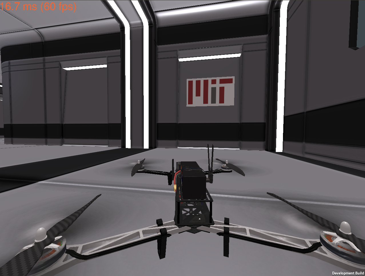

Since we linked your controller_pkg from your lab3 team-submissions, your controller should be running with the gains you found in lab3. Feel free to further tune the gains in ~/vnav/ws/lab4/src/controller_pkg/config/params.yaml.

Before you start coding, let’s take a look at the big picture. This is the system we’re trying to construct: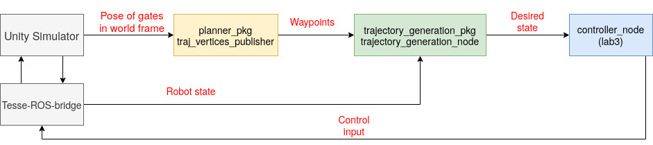

Coding – Part 0

As a warm up exercise, let’s just fly and hover at the first gate! Follow the instructions for Part 0 inside planner_pkg/src/simple_traj_planner.cpp.

To run your code, use the following commands:

# terminal 1
# run the simulator
cd ~/vnav/tesse/lab4
./lab4.x86_64

# terminal 2
# launches the bridge between tesse and ros2
# NOTE: make sure you always start the bridge AFTER the simulator
ros2 launch tesse_ros_bridge tesse_quadrotor_bridge.launch.yaml

# terminal 3
# launches the controller_node, traj_vertices_publisher, simple_traj_planner
ros2 launch planner_pkg static_point_test.launch.py

• Hint: you can press r to respawn your quadcopter
• Hint: review the handout from lab 3 if you have trouble running the simulator.

Coding – Parts 1.1, 1.2, and 1.3

Next, let’s implement the rest of the stack. Follow the instructions for Parts 1.1, 1.2, and 1.3 in trajectory_generation_pkg/src/trajectory_generation_node.cpp to get your quadcopter ready for drone racing!

This node will subscribe to the waypoints published and use them for trajectory optimization using the mav_trajectory_generation library, and then based on the trajectory, publish the desired state at time t to your controller.

• Hint: use vertex.addConstraint(POSITION, position) where position is of type Eigen::Vector3d to enforce a waypoint position.
• Hint: use vertex.addConstraint(ORIENTATION, yaw) where yaw is a double to enforce a waypoint yaw.
• Hint: remember angle wraps around 2$\pi$. Be careful!
• Hint: for the ending waypoint for position use end_vertex.makeStartOrEnd as seen with the starting waypoint instead of vertex.addConstraint as you would do for the other waypoints.

To run your code, use the following commands:

# terminal 1
# run the simulator
cd ~/vnav/tesse/lab4
./lab4.x86_64

# terminal 2
# launches the bridge between tesse and ros2
# NOTE: make sure you always start the bridge AFTER the simulator
ros2 launch tesse_ros_bridge tesse_quadrotor_bridge.launch.yaml

# terminal 3
# launches the controller_node and trajectory_generation_node (i.e., trajectory follower)
ros2 launch trajectory_generation traj_following.launch.py

# terminal 4
# launches traj_vertices_publisher node (i.e., waypoint publisher)
ros2 launch planner_pkg traj_gen.launch.py

If everything is working well, your drone should be gracefully going through each gate like this

Note: If the quadcopter flips over after launching the trajectory follower, press r in the Unity window to respwan, the quadcopter should just go back to the starting position.

Recording a Video and ROS2 Bag

Once you have your drone racing, you will need to submit a video and a ROS2 bag recording of your best trial.

To take a video, ideally use a screen recorder of your choice. If this isn’t working with your setup, you make take a high quality video of your screen with a phone.

To collect a ROS2 bag recording, use the following command (i.e., it only records the /current_state and /desired_state topics):

ros2 bag record /current_state /desired_state

Note that a ROS2 bag recording is a folder with a metadata.yaml and .db3 file(s) – i.e., it is no longer a single .bag files as in ROS1.

Upload the both the video and ROS2 bag folder to Google Drive or Dropbox, generate two publicly viewable links, and place them in a textfile called links.txt within your team-submissions/lab4 folder.

Submitting your code

Navigate to your submisison directory:

cd ~/vnav/team-submissions/lab4

Sanity check the correct files/folders are in the lab4 submission directory:

$ ls
links.txt  planner_pkg  trajectory_generation_pkg

Add these files to your submission repo, commit, and push:

git add links.txt
git add planner_pkg
git add trajectory_generation
git commit -m "YOUR MESSAGE HERE"
git push

Confirm the submitted files appear correctly in your team’s submission repo.

[Optional] Faster, faster (Extra credit: 15 pts)

How can you make the drone go faster? We will award extra credit to the fastest 3 teams! Current record is 10.3s, achieved by Nikhil Singhal, Fernando Herrera and Chris Chang in 2020.

[Optional] Provide feedback (Extra credit: 3 pts)

This assignment involved a lot of code rewriting, so it is possible something is confusing or unclear. We want your feedback so we can improve this assignment (and the class overall) for future offerings. If you provide actionable feedback to the Google Form link, you can get up to 3 pts of extra credit. Feedback can be positive, negative, or something in between – the important thing is your feedback is actionable (i.e., “I did’t like X” is vague, hard to address, and thus not actionable).

The Google Form is pinned in the course Piazza (we do not want to post the link publically, which is why it is not provided here).

Note that we cannot give extra points for anonymous feedback while maintaining your anonymity. That being said, you are still encouraged to provide anonymous feedback if you’d like!