Exercises
- Submission
- 👤 Individual
- 👥 Team
- Update the lab codebase
- Feature Tracking and Matching
- Descriptor-based Feature Matching
- 📨 Deliverable 3 - Feature Descriptors (SIFT) [20 pts]
- 📨 Deliverable 4 - Descriptor-based Feature Matching [10 pts]
- 📨 Deliverable 5 - Keypoint Matching Quality [10 pts]
- 📨 Deliverable 6 - Comparing Feature Matching Algorithms on Real Data [20 pts + optional 10 pts]
- 📨 Deliverable 7 - Feature Tracking: Lucas Kanade Tracker [20 pts]
- 📨 [Optional] Deliverable 8 - Optical Flow [+10 pts]
Submission
To submit your solutions create a folder called lab5 and push one or more file to your repository with your answers.
Individual
Please submit the deliverables to Gradescope. For math-related questions only typeset PDF files are allowed (e.g., using Latex, Word, Markdown).
Team
Please push the source code for the entire package to the folder lab5 of the team repository. For the tables and discussion questions, please push a PDF to the lab5 folder of your team repository.
Deadline
Deadline: the VNAV staff will clone your repository on October 9th at 1 PM EDT.
👤 Individual
📨 Deliverable 1 - Practice with Perspective Projection [10 pts]
Consider a sphere with radius $r$ centered at $[0\ 0\ d]$ with respect to the camera coordinate frame (centered at the optical center and with axis oriented as discussed in class). Assume $d > r + 1$ and assume that the camera has principal point at $(0,0)$, focal length equal to 1, pixel sizes $s_x = s_y = 1$ and zero skew $s_\theta = 0$ (see lecture notes for notation) the following exercises:
- Derive the equation describing the projection of the sphere onto the image plane.
- Hint: Think about what shape you expect the projection on the image plane to be, and then derive a characterisitic equation for that shape in the image plane coordinates $u,v$ along with $r$ and $d$.
- Discuss what the projection becomes when the center of the sphere is at an arbitrary location, not necessarily along the optical axis. What is the shape of the projection?
📨 Deliverable 2 - Vanishing Points [10 pts]
Consider two 3D lines that are parallel to each other. As we have seen in the lectures, lines that are parallel in 3D may project to intersecting lines on the image plane. The pixel at which two 3D parallel lines intersect in the image plane is called a vanishing point. Assume a camera with principal point at (0,0), focal length equal to 1, pixel sizes $s_x = s_y = 1$ and zero skew $s_\theta = 0$ (see lecture notes for notation). Complete the following exercises:
- Derive the generic expression of the vanishing point corresponding to two parallel 3D lines.
- Find (and prove mathematically) a condition under which 3D parallel lines remain parallel in the image plane.
- Hint: For both 1. and 2. you may use two different approaches:
- Algebraic approach: a 3D line can be written as a set of points $p(\lambda) = p_0 + \lambda u$ where $p_0 \in \mathbb{R}^3$ is a point on the line, $u \in \mathbb{R}^3$ is a unit vector along the direction of the line, and $\lambda \in \mathbb{R}$.
- Geometric approach: the projection of a 3D line can be understood as the intersection beetween two planes.
👥 Team
Update the lab codebase
First, update your stencil code repo:
cd ~/vnav/starter-code
git pull
Copy the contents of the lab5 directory into your team submissions repo, e.g.
cp -r ~/vnav/starter-code/lab5 ~/vnav/team-submissions/lab5
If you want to use the directory structure introduced in Lab 4, then make a lab5 directory in ~/vnav/ws and link your lab5 directory from the team-submissions repo.
Feature Tracking and Matching
Feature tracking between images is a fundamental module in many computer vision applications, as it allows us both to triangulate points in the scene and, at the same time, estimate the position and orientation of the camera from frame to frame (you will learn how to do so in subsequent lectures).
Descriptor-based Feature Matching
Feature Detection (SIFT)
Feature detection consists of extracting keypoints (pixel locations) in an image. In order to track features reliably from frame to frame, we need to specify what is a good feature to detect.
The ideal features in an image are the ones that have the following properties:
- Repeatability: the same feature can be found in several images despite geometric (i.e. rotations, scale changes, etc) and photometric transformations (i.e. changes in brightness).
- Saliency: each feature has a distinctive description. Otherwise, matching between features is difficult if all features look the same.
- Compactness and efficiency: fewer features than image pixels.
- Locality: a feature occupies a relatively small area of the image, making it robust to clutter and occlusion.
As you have seen in the lecture, one very successful feature detector is SIFT (Scale Invariant Feature Transform), which is not only invariant to image rotations, but also to scale changes of the image.
Let us now use SIFT to detect keypoints in an image to see the actual output.
We want you to get familiar with state-of-the-art feature detectors, so we will avoid having you re-implement the detectors themselves and focus instead on their comparison. Refer to the tutorials in OpenCV for the different algorithms we will be using for more details. For example, SIFT is detailed here and its OpenCV API is defined here. You will need to search through the OpenCV documentation for details on the other descriptors and methods mentioned in this handout.
📨 Deliverable 3 - Feature Descriptors (SIFT) [20 pts]
We provide you with skeleton code for the base class FeatureTracker that provides an abstraction layer for all feature trackers. Furthermore, we give you two empty structures for the SIFT and AKAZE methods that derive from the class FeatureTracker.
Inside the lab5 folder, we provide you with two images box.png and box_in_scene.png (inside the images folder).
We will first ask you to extract keypoints from both images using SIFT. For that, we refer you to the skeleton code in the src folder named track_features.cpp. Follow the instructions written in the comments; specifically, you will need to complete:
- The stub
SiftFeatureTracker::detectKeypoints()andSiftFeatureTracker::describeKeypoints()inlab5/src/sift_feature_tracker.cpp - The first part of
FeatureTracker::trackFeatures()inlab5/src/feature_tracker.cpp
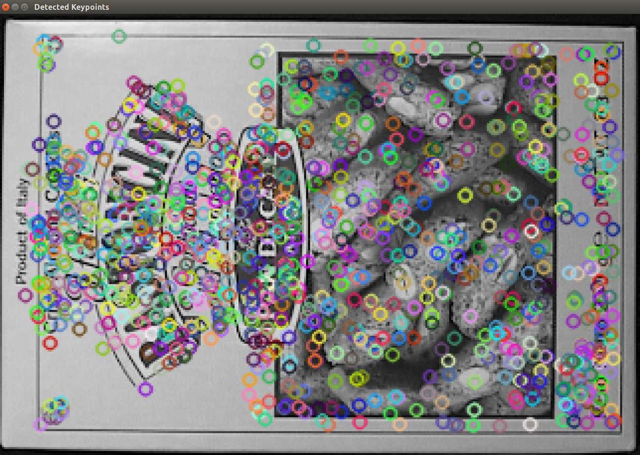
Once you have implemented SIFT and built the lab5 package, you can test it by running:
ros2 launch lab_5 two_frames_tracking.launch.yaml descriptor:=SIFT # note you can change the descriptor later
Your code should be able to plot a figure like the one below (keypoints you detected should not necessarily coincide with the ones in the figure):
Now that we have detected keypoints in each image, we need to find a way to uniquely identify these to subsequently match features from frame to frame. There are many feature descriptors described in the literature, and while we will not review all of them, they all rely on a similar principle: using the pixel intensities around the detected keypoint to describe the feature. Descriptors are multidimensional and are typically represented by an array.
Follow the skeleton code in src to compute the descriptors for all the extracted keypoints.
- Hint: In OpenCV, SIFT and the other descriptors we will look at are children of the “Feature2D” class. We provide you with a SIFT
detectorobject, so look at the Feature2D “Public Member Functions” documentation to determine which command you need to detect keypoints and get their descriptors.
📨 Deliverable 4 - Descriptor-based Feature Matching [10 pts]
With the pairs of keypoint detections and their respective descriptors, we are ready to start matching keypoints between two images. It is possible to match keypoints just by using a brute force approach. Nevertheless, since descriptors can have high-dimensionality, it is advised to use faster techniques.
In this exercise, we will ask you to use the FLANN (Fast Approximate Nearest Neighbor Search Library), which provides instead a fast implementation for finding the nearest neighbor. This will be useful for the rest of the problem set, when we will use the code in video sequences.
- What is the dimension of the SIFT descriptors you computed?
- Compute and plot the matches that you found from the box.png image to the box_in_scene.png.
- You might notice that naively matching features results in a significant amount of false positives (outliers). There are different techniques to minimize this issue. The one proposed by the authors of SIFT was to calculate the best two matches for a given descriptor and calculate the ratio between their distances:
Match1.distance < 0.8 * Match2.distanceThis ensures that we do not consider descriptors that have been ambiguously matched to multiple descriptors in the target image. Here we used the threshold value that the SIFT authors proposed (0.8). - Compute and plot the matches that you found from the box.png image to the box_in_scene.png after applying the filter that we just described. You should notice a significant reduction of outliers.
Specifically, you will need to complete:
- The stub
SiftFeatureTracker::matchDescriptors()insift_feature_tracker.cpp - The second part of
FeatureTracker::trackFeatures()infeature_tracker.cpp
📨 Deliverable 5 - Keypoint Matching Quality [10 pts]
Excellent! Now that we have the matches between keypoints in both images, we can apply many cool algorithms that you will see in subsequent lectures.
For now, let us just use a blackbox function which, given the keypoints correspondences from image to image, is capable of deciding whether some matches are considered outliers.
- Using the function we gave you in
feature_tracker.cpp, compute and plot the inlier and outlier matches, such as in the following figure: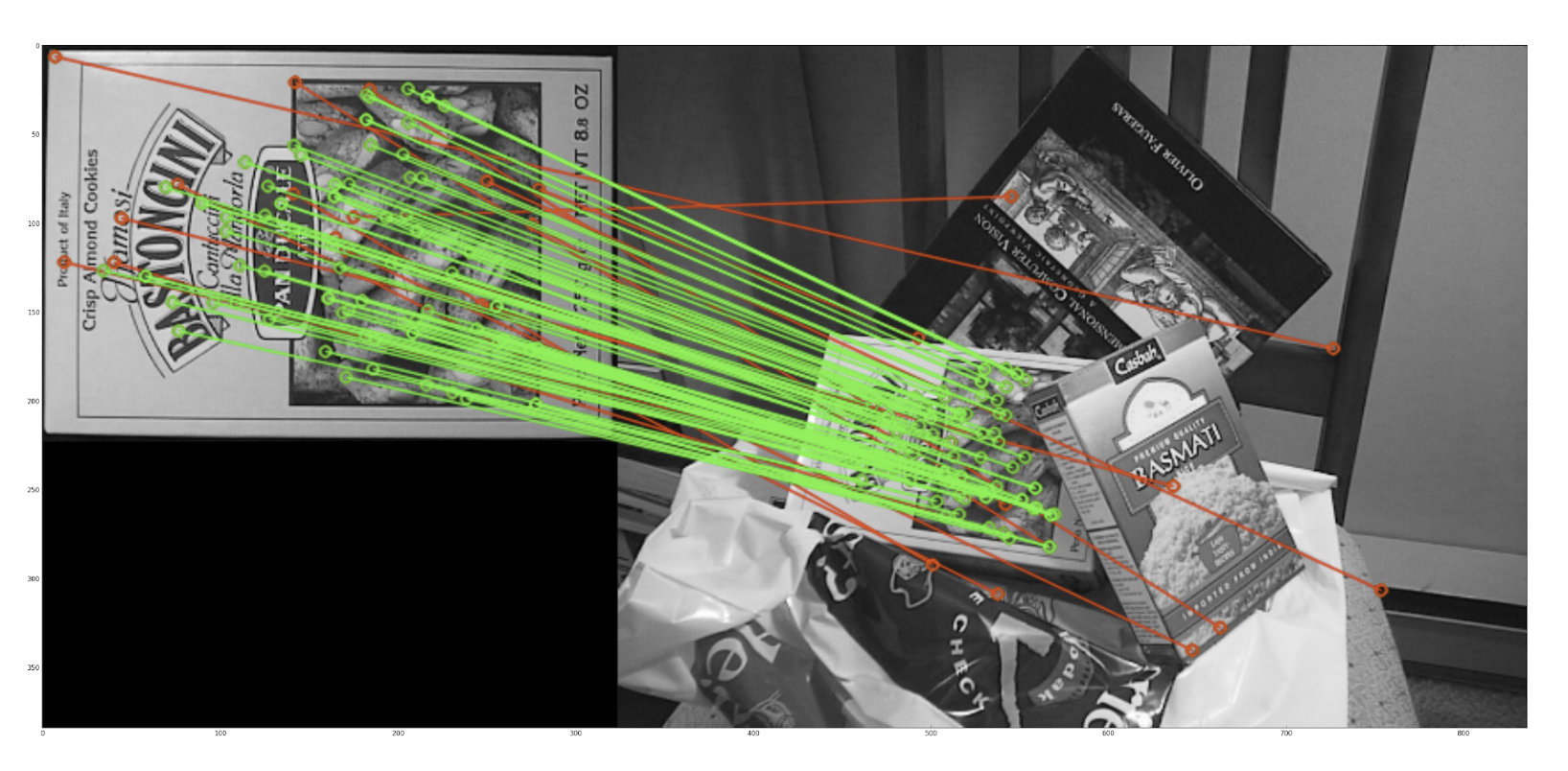
- Hint: Note that
FeatureTracker::inlierMaskComputationcomputes an inlier mask of typestd::vector<uchar>, but forcv::drawMatchesyou will need astd::vector<char>. You can go from one to the other by using:
std::vector<char> char_inlier_mask{inlier_mask.begin(), inlier_mask.end()}; - Hint: You will need to call the
cv::drawMatchesfunction twice, first to plot the everything in red (usingcv::Scalar(0,0,255)as the color), and then again to plot inliers in green (using the inlier mask andcv::Scalar(0,255,0)). The second time, you will need to use theDrawMatchesFlags::DRAW_OVER_OUTIMGflag to draw on top of the first output. To combine flags for thecv::drawMatchesfunction, use the bitwise-or operator:DrawMatchesFlags::NOT_DRAW_SINGLE_POINTS | DrawMatchesFlags::DRAW_OVER_OUTIMG
- Hint: Note that
- Now, we can calculate useful statistics to compare feature tracking algorithms. First, let’s compute statistics for SIFT. The code for computing the statistics is already included in the skeleton file. You just need to use the appropriate functions to print them out. Submit a table similar to the following for SIFT (you might not get the same results, but they should be fairly similar):
| Statistics | Approach | |
|---|---|---|
| SIFT | ... | |
| # of Keypoints in Img 1 | 603 | |
| # of Keypoints in Img 2 | 969 | |
| # of Matches | 603 | |
| # of Good Matches | 93 | |
| # of Inliers | 78 | |
| Inlier Ratio | 83.9% | |
📨 Deliverable 6 - Comparing Feature Matching Algorithms on Real Data [20 pts + optional 10 pts]
The most common algorithms for feature matching use different detection, description, and matching techniques. We’ll now try different techniques and see how they compare against one another:
6.a. Pair of frames
Fill the previous table with results for other feature tracking algorithms. We ask that you complete the table using the following additional algorithms:
- Hint: The AKAZE and ORB functions can be implemented similarly to SIFT, except that the FLANN matcher must be initialized with a new parameter like this:
FlannBasedMatcher matcher(new flann::LshIndexParams(20, 10, 2));. This is not necessarily the best solution for ORB and AKAZE however, so we encourage you to look into other methods (e.g. the Brute-Force matcher instead of the FLANN matcher) if you have time.
We have provided method stubs in the corresponding header files for you to implement in the CPP files. Please refer to the OpenCV documentation, tutorials, and C++ API when filling them in. You are encouraged to modify the default parameters used by the features extractors and matchers. A complete answer to this deliverable should include a brief discussion of what you tried and what worked the best.
ATTENTION.
NOTE: If you have the issue "Unknown interpolation method in function 'resize'" for your ORB feature tracker, explicitly set the number of levels in the ORB detector to 1 see OpenCV API here)
By now, you should have four algorithms, with their pros and cons, capable of tracking features between frames.
- Hint: It is normal for some descriptors to perform worse than others, especially on this pair of images – in fact, some may do very poorly, so don’t worry if you observe this.
6.b. Real Datasets
Let us now use an actual video sequence to track features from frame to frame and push these algorithms to their limit!
We have provided you with a set of datasets in rosbag format here. Please download the following datasets, which are the two “easiest” ones:
30fps_424x240_2018-10-01-18-35-06.bagvnav-lab5-smooth-trajectory.bag
Put the downloaded folders in the lab5/bags directory, and then make sure to build again.
Testing other datasets may help you to identify the relative strengths and weaknesses of the descriptors, but this is not required.
We also provide you with a roslaunch file that executes two ROS nodes:
ros2 launch lab_5 video_tracking.launch.yaml bag_name:=<name of bag to test> # Alternatively, you can set the absolute path to the bag with path_to_dataset:=<path>
- One node plays the rosbag for the dataset
- The other node subscribes to the image stream and is meant to compute the statistics to fill the table below
You will need to first specify in the launch file the path to your downloaded dataset. Once you’re done, you should get something like this:
- Hint: You may need to change your plotting code in
FeatureTracker::trackFeaturesto callcv::waitKey(10)instead ofcv::waitKey(0)after imshow in order to get the video to play continuously instead of frame-by-frame on every keypress.
Finally, we ask you to summarize your results in one table for each dataset and asnwer some questions:
- Compute the average (over the images in each dataset) of the statistics on the table below for the different datasets and approaches. You are free to use whatever parameters you find result in the largest number of inliers.
| Statistics | Approach for Dataset X | |||
|---|---|---|---|---|
| SIFT | AKAZE | ORB | BRISK | |
| # of Keypoints in Img 1 | ... | ... | ... | ... |
| # of Keypoints in Img 2 | ... | ... | ... | ... |
| # of Matches | ... | ... | ... | ... |
| # of Good Matches | ... | ... | ... | ... |
| # of Inliers | ... | ... | ... | ... |
| Inlier Ratio | ...% | ...% | ...% | ...% |
What conclusions can you draw about the capabilities of the different approaches? Please make reference to what you have tested and observed.
- Hint: We don’t expect long answers, there aren’t specific answers we are looking for, and you don’t need to answer every suggested question below! We are just looking for a few sentences that point out the main differences you noticed and that are supported by your table/plots/observations.
Some example questions to consider: - Which descriptors result in more/fewer keypoints?
- How do they the descriptors differ in ratios of good matches and inliers?
- Are some feature extractors or matchers faster than others?
- What applications are they each best suited for? (e.g. when does speed vs quality matter)
📨 Deliverable 7 - Feature Tracking: Lucas Kanade Tracker [20 pts]
So far we have worked with descriptor-based matching approaches. As you have seen, these approaches match features by simply comparing their descriptors. Alternatively, feature tracking methods use the fact that, when recording a video sequence, a feature will not move much from frame to frame. We will now use the most well-known differential feature tracker, also known as Lucas-Kanade (LK) Tracker.
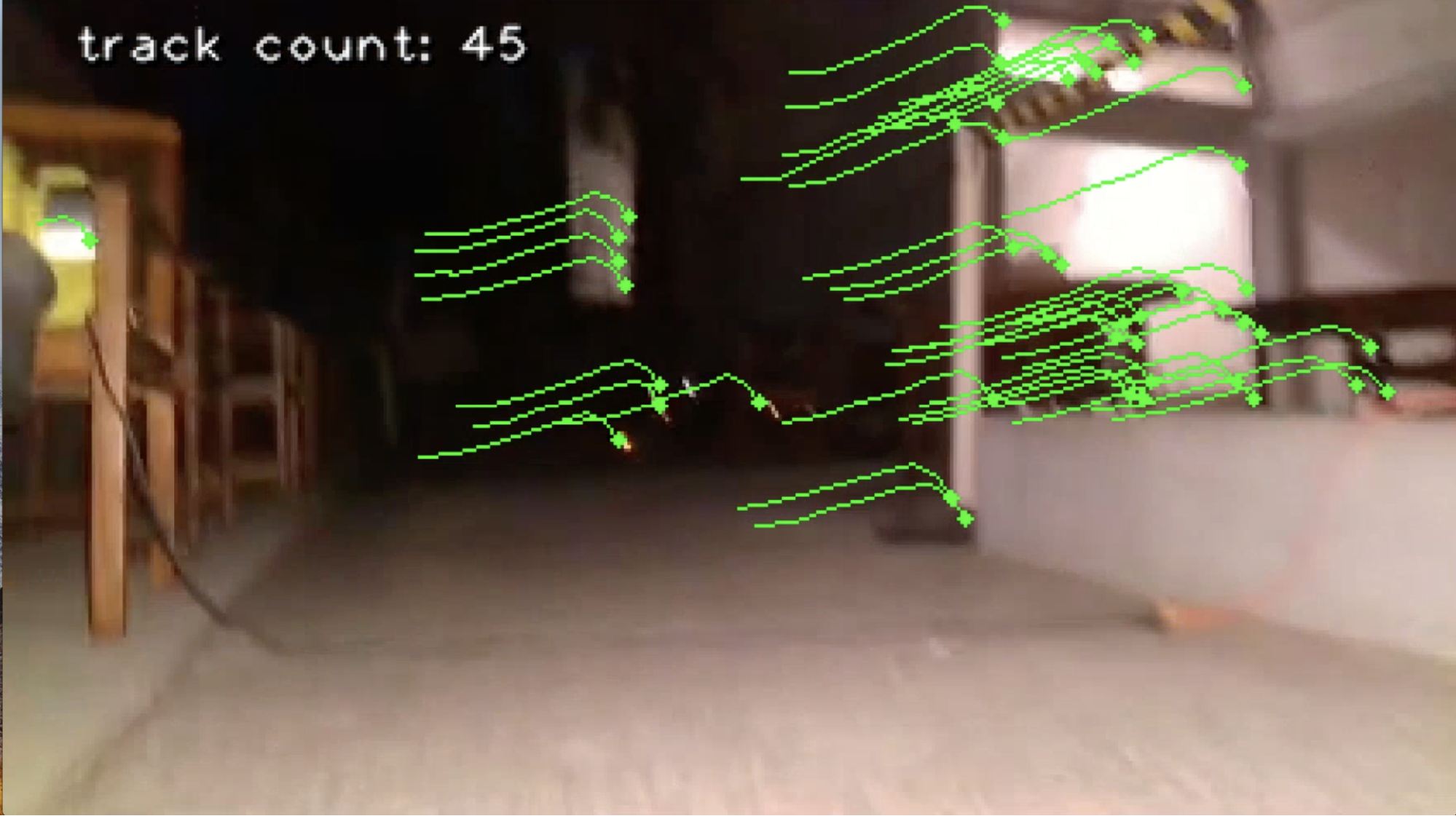
- Using OpenCV’s documentation and the C++ API for the LK tracker, track features for the video sequences we provided you by using the Harris corner detector (like here). Show the feature tracks at a given frame extracted when using the Harris corners, such as this:
- Add an extra entry to the table used in Deliverable 6. using the Harris + LK tracker that you implemented.
- What assumption about the features does the LK tracker rely on?
- Comment on the different results you observe between the table in this section and the one you computed in the other sections.
Hint: You will need to convert the image to grayscale with
cv::cvtColorand will want to look into the documentation forcv::goodFeaturesToTrackandcv::calcOpticalFlowPyrLK. The rest of the trackFeatures() function should be mostly familiar feature matching and inlier mask computation similar to the previous sections. Also note that thestatusvector from calcOpticalFlowPyrLK indicates the matches.Hint: For the show() method, you will just need to create a copy of the input frame and then make a loop that calls
cv::lineandcv::circlewith correct arguments before callingimshow.
📨 [Optional] Deliverable 8 - Optical Flow [+10 pts]
LK tracker estimates the optical flow for sparse points in the image. Alternatively, dense approaches try to estimate the optical flow for the whole image. Try to calculate your own optical flow, or the flow of a video of your choice, using Farneback’s algorithm.
- Hint: Take a look at this tutorial, specifically the section on dense optical flow. Please post on piazza if you run into any issues or get stuck anywhere.