Exercises

Submission
👤 Individual
1. 📨 Deliverable 1 - Accounting for Measurement Covariances in Nonlinear Least Squares [10 pts]
2. 📨 Deliverable 2 - Practice with Lie Groups (35 pts)
👥 Team

Submission

To submit your solutions create a folder called lab7 and push one or more file to your repository with your answers (it can be plain text, markdown, pdf or whatever other format is reasonably easy to read)

Individual

Please push the deliverables into your personal repository. Since there are mostly math-related questions, only typeset PDF files are accepted (e.g., using Latex, Word, Markdown).

Team

Please push the source code for the entire package to the folder lab7 of the team repository. Additionally, please also include a PDF file in your lab7 folder that contains all the text files and images (see “Summary of Team Deliverables” at the end of this page for details).

Deadline

Deadline: the VNAV staff will clone your repository on October 25th at 1 PM EDT.

👤 Individual

📨 Deliverable 1 - Accounting for Measurement Covariances in Nonlinear Least Squares [10 pts]

Consider the following cost function $f(x) = r(x)^T W r(x)$ where $r:\mathbb{R}^n \rightarrow \mathbb{R}^m$ and $W$ is an $m \times m$ positive-definite matrix.

Express this optimization problem as a standard (non-weighted) nonlinear least squares problem when $W$ is diagonal.
Answer 1. when $W$ is not necessarily diagonal.
Derive the normal equations for $\min r(x)^T W r(x)$ in an iteration of Gauss-Newton.

📨 Deliverable 2 - Practice with Lie Groups (35 pts)

Consider the case in which we are given $n$ poses $T_i \in \SE{3}$, $i=1,\ldots,n$ and we are looking for the average pose that minimizes the average (squared) chordal distance:

\[ T^\star = \argmin_{T\in\SE{3}} \frac{1}{n} \sum_{i=1}^n \|T-T_i \|^2_F \]

Can you compute a closed-form expression for $T^\star$?
- Hint: Review Lecture 16 notes for inspirations on Matrix / Algebraic manipulations.
How does the previous answer change when we adopt a weighted chordal distance \[ T^\star = \argmin_{T\in\SE{3}} \frac{1}{n} \sum_{i=1}^n \| T-T_i \|^2_{\Omega_i} \tag{1} \] Where, for a matrix $M$, we defined $\|M\|^2_{\Omega} = \trace(M\Omega M\tran)$ and the weight matrix is defined as: \[ \Omega_i = \begin{bmatrix} \omega_i I_3 & 0_3 \\ 0_3\tran & \varrho_i \end{bmatrix} \] $I$ here denotes the $3 \times 3$ identity matrix.
How do $\omega_i$ and $\varrho_i$ affect the average pose? For instance, what happens if for a single $i$ the coefficients $\omega_i$ and $\varrho_i$ are very large?
Prove that the minimization of the weighted chordal distance (1) is a maximum likelihood estimator given measurements where $R$ is Langevin and $t$ is Gaussian. In other words prove that, the solution $T^*$ of (1) satisfies \[ T^\star = \argmax_{T\in\SE{3}} \prod_{i=1}^n P(T_i \mid T) \] Where $T_i \in \SE{3}, i = 1,\ldots,n$ are $n$ i.i.d. samples where $T_i = (R_i, t_i)$ \[P(R_i \mid R) = \mathrm{Langevin}(R, \omega_i) \] \[P(t_i \mid t) = \mathrm{Gaussian}(t, \frac{1}{\rho_i} I) \] $I$ here denotes the $3 \times 3$ identity matrix.
Now, let’s try to find the above maximum likelihood estimate through local search. Express this problem as a least squares problem assuming the concentration parameters are $\omega_i = 1$. Derive the Gauss-Newton and Levenberg-Marquardt steps for this problem.
[Optional] Write out the explicit expression for the Jacobians. (+ 5 pts)

👥 Team

GTSAM Preliminaries

While we do a very practical introduction to GTSAM (Georgia Tech Smoothing And Mapping) below, this does not replace the primer written by Frank Dellaert: https://gtsam.org/tutorials/intro.html

We will give you pointers to the relevant sections in this document to avoid having a long handout, but if in doubt either refer to this guide or to the GTSAM code itself.

GTSAM was developed to solve estimation problems. In particular, problems that can be formulated in terms of probability densities over a set of variables ($X$) for which we only have (noisy) measurements ($Z$)). Since we only care about the most likely values for X given the measurements Z, we use the Maximum A-Posteriori (MAP) estimator, which, as you have seen in class, tries to solve the following problem:

\[\argmax_X p(z_1,\ldots,z_n \mid X)p(X)\]

Assuming that we have nonlinear measurements with additive Gaussian noise, we can formulate this problem as a nonlinear Least Squares problem (after taking the negative log likelihood of the previous expression and simplifying):

\[X_{MAP} = \argmin_X \sum_i \|h_i(X_i) - z_i\|_{\Sigma_i}^2 \tag{2}\]

Where we sum multiple residuals (error between the measurements $z_i$ and what would be the expected measurement $h_i(X_i)$ given a subset of variable assignments $X_i$

GTSAM makes use of a probabilistic graphical model known as a Factor Graph, which is a model to visualize and reason over problems similar to the one in eq. (2). While we have a more formal introduction to factor graphs next week, for now you can think about factor graphs as a way to describe a least squares problem.

In particular, each summand in eq (2) is a “factor”, and the overall objective forms a factor graph. Therefore, if we want to instantiate problem (2) in GTSAM, we will need the following objects:

NonlinearFactorGraph: this object allows for building the problem by adding a set of factors. Most important functions that this class offers are:
- add: adds a factor to the factor graph. A factor graph is built by adding multiple factors between variables or for single variables. A factor is just a function of the variables and the measurements which gives the mismatch (error) between both. Note: You might sometimes see GTSAM using instead of add, the function emplace_shared (both are valid but have different calls, if you are not familiar with templates in C++ use add).
- print: to print the factors that make the underlying factor graph.
Symbol and Key: Symbols and Keys are used to index variables in the factor graph (though internally every variable has a key); a Key is just a typedef for an integer of size uint64_t.
Values: This is the actual numeric values for the variables that you are using in the optimization problem. Since we will be using iterative solvers, an initial estimate must be provided, which is given as a set of initial values. The result of the optimization problem will also be a set of values for your variables.
Geometric entities:
- Rot3: A rotation matrix.
- Point2 and Point3: 2D or 3D positions.
- Pose3: A generic transformation matrix with a Rot3 rotation and a Point3 translation.
Solvers: GTSAM implements different optimization algorithms amongst which the most relevant for us are:
- GaussNewtonOptimizer
- LevenbergMarquardtOptimizer

// Simple example gtsam snippet 

// Create an empty nonlinear factor graph 
gtsam::NonlinearFactorGraph nfg; 

// Create values 
Values values; 

// Create a factor (in this case, a between factor: which provides an SE3 measurement between 2 nodes)
//// Between factor connecting nodes with key 0 and key 1 where measurement of relative pose between two nodes 
//// is transformation with rotation 1, 0, 0, 0 (qx, qy, qz, qw) and translation 1, 0, 0 (x, y, z)
gtsam::BetweenFactor<gtsam::Pose3> between_factor(0, 1, gtsam::Pose3(gtsam::Rot3(1, 0, 0, 0), gtsam::Point3(1, 0, 0)));

// Add factor to factor graph 
nfg.add(between_factor);

// Add initial estimates 
//// We have 2 poses as nodes in the factor graph. 
//// Adding identity pose as initial guess
values.insert(0, gtsam::Pose3()); // Initial estimate for node with key 0
values.insert(0, gtsam::Pose3()); // Initial estimate for node with key 1

//// Optimize with Gauss-Newton:
gtsam::GaussNewtonParams parameters;
// Modify the max number of iterations to see the overall improvement.
parameters.setMaxIterations(6);
parameters.setAbsoluteErrorTol(1e-06);
// Print per iteration.
parameters.setVerbosity("ERROR");
// Create the optimizer GaussNewtonOptimizer given the parameters
// above , the initial values and the graph.
gtsam::GaussNewtonOptimizer optimizer(nfg, values, parameters);
// Finally, Optimize!
values = optimizer.optimize();
// To print estimates after optimization 
values.print("\n optimized. \n");

//// Similarly, to optimize with Levenberg-Marquardt:
gtsam::LevenbergMarquardtParams parameters;
gtsam::LevenbergMarquardtOptimizer optimizer(nfg, values, parameters);
values = optimizer.optimize();

Setting up

Install packages that you might need:
```
sudo apt-get install libtbb-dev
```
Add new packages to your catkin workspace using wstool:
```
cd {VNAV_HOME}/vnav_ws/src/
cp -r {VNAV_HOME}/Labs/lab7 ./
wstool merge --merge-replace {VNAV_HOME}/vnav_ws/src/lab7/install/lab_7.rosinstall -y
wstool update
```
Note you might get duplicated packages with previous labs in your workspace. Please manually remove the duplicates. Note this might take 15min, GTSAM is quite large.
Build lab_7:
```
catkin build gtsam
catkin build `lab_7`
```
Note Build gtsam catkin build gtsam before building lab_7. Remember to source your workspace:
```
source {VNAV_HOME}/vnav_ws/devel/setup.bash
```

📨 Deliverable 1 - GTSAM Introduction [10 pts]

The best introduction to GTSAM coding style is by far the hands-on introduction written by Frank Dellaert (creator of GTSAM). We will follow it as a first step to get familiar with the calls and variables that GTSAM uses.

In this section, we will be following the hands-on guide up to and including section 3. You should not be spending too much time here writing the code as all the answer should be straight out of the guide. You should, however, use this exercise as an opportunity to familiarize yourself to the API of GTSAM, along with the basics, such as how a pose is defined, and what a factor is.

Open up deliverable_1.cpp and follow the hands-on guid to add odometry factors (between factors) in 1a. Then add “GPS” like factors in 1b. (Even though we completed the definition of the UnaryFactor here for you, pay attention to how it was defined!). And finally, create the (deliberately) inaccurate initial estimate in 1c.

In this lab, we will be using different executables, one for each deliverable, and we are not using more than one node at a time, therefore we will just use rosrun. To run rosrun, you need first to launch roscore in a terminal.

roscore

rosrun lab_7 deliverable_1

to run the code. Provide the values before and after optimization and save to a file called deliverable_1.txt in your submission folder.

📨 Deliverable 2 - GTSAM 3D Pose Estimation [10 pts]

Let’s switch over to 3D. To do this, you will need to use the Pose3 class instead of a Pose2. The provided function generateOdometryMeasurements create a large number of odometry measurements (50-500). We want to use these odometry measurements to find the pose estimates of the poses in the pose graph. In deliverable_2_3.cpp, fill in 2a. and 2b. to add the odometry measurements as Between Factors in SE3 and also constrain the initial pose with a Prior Factor
We provide you with a configuration file for Rviz, you can use it by running rviz -d /path/to/lab_7.rviz. You will see the following:
- Ground-Truth trajectory.
- Noisy trajectory (used to create the odometry measurements)
- Initial estimate of the actual trajectory.
- Optimized trajectory after estimation.
Using the parameter setMaxIterations for the GaussNewtonOptimizer, show the optimized trajectory after 1, 3 and 6 iterations. Take screen shots of the rviz visualization and add to your submissions folder.

📨 Deliverable 3 - Making a Motion Capture Factor in GTSAM [15 pts]

Let us now fuse the information coming from a Motion Capture system (you can think of this as an indoor 3D GPS system). To do this, we provide you with the function generateMoCapMeasurements which simulates noisy measurements of the position of the robot for some poses. To use this new sensor information, you need to implement a new factor.

In deliverable_2_3.h fill in 3a. Derive and complete the new MoCapPosition3Factor which takes a Point3 position of the drone/robot as measurement and calculates the error with respect to our estimate of the pose of the robot (Pose3). Get inspiration from the Robot Localization example in the hands-on introduction of GTSAM, since this functions similarly to the UnaryFactor except we are now feeding in 3D positions instead of 2D positions.
In deliberable_2_3.cpp fill in 3b. to add the motion caption measurements. Remember to set static constexpr bool use_mocap = true; on line 273.
Similarly to before, show using the setMaxIterations for the GaussNewtonOptimizer the optimized trajectory after 1, 3 and 6 iterations. Take screen shots and submit.

Few things to node when defining a new factor:

Jacobians: usually represented by a matrix named H.
Error functions: in GTSAM every factor has to define what the error is given the variable and the measurement. In practice, you must always define the function evaluateError. Such a function has to have as parameters not only the current value for a variable (to be able to calculate the error against the measurement) but also the Jacobian of this error function with respect to the variable. Have a look at section 3.2 Defining Custom Factors in here for reference on the actual API used by GTSAM to code your own factor.

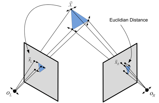
📨 Deliverable 4 - GTSAM to solve Computer Vision problems [20 pts]

GTSAM is particularly useful when we need to solve optimization problems that we frequently encounter in State Estimation using Visual information.

We have seen in previous lectures and labs how to find the relative transformation between two camera poses given their images using a 5 or 8-point method. Nevertheless, we have also seen that this is not the most accurate way of estimating the trajectory of the drone and ML estimation suggest that the best estimate can be computed using Bundle Adjustment.

We will now use the optimization in GTSAM that we just learned about in order to calculate both the poses of a camera and the positions of the landmarks observed from these cameras via bundle adjustment.

Bundle adjustment (Source)

Bundle Adjustment refers to the problem for which we have a set of 2D correspondences for multiple frames and we want to estimate the poses of the cameras that took the frames as well as the 3D landmarks corresponding to the keypoins. Since a given bundle of 3D rays from the camera origins to the world will unlikely intersect on the actual 3D point $X_j$, we try instead to find the set of camera poses $P_i$ and landmark positions $X_j$ that minimize the so-called re-projection error. This error accounts for the distance between the measured pixel coordinates of a keypoint $x_{ij}$ and the actual point in the image where the corresponding 3D landmark should reproject to according to the current state configuration (camera poses $P_i$ and landmark positions $X_j$). Minimizing the sum of all these reprojection errors yields the most likely configuration of camera poses and landmarks positions that resulted in the given keypoint measurements. (Review Example 2 from Lecture 16 notes. )

Let us try to solve a Bundle Adjustment problem. We provide you with a set of simulated camera poses and 2D measurements of certain 3D landmarks in the world. In other words, we give you the 2D correspondences between keypoints in all images (the ones you would have extracted using SIFT for example). We also provide you with the calibration matrix K of the camera, which you would have otherwise computed previously by calibrating the camera.

In deliverable_4.cpp, we provide you with the steps and data to solve a simple Bundle Adjustment problem. We ask you to

Solve the Bundle Adjustment Problem: print and report your initial and final optimized result. Check out the documentation on GenericProjectionFactor and example usage
Visualize in Rviz (rviz -d deliverable_4.rviz):
- The 3D positions of the landmarks before/after optimization.
- The frame of reference of the cameras before/after optimization.
- The ground-truth of the above variables (camera poses + landmarks).
Take a screenshot of your visualization and add to submissions folder.

Note that in the instructions we say to use the character ‘l’ to symbolize landmarks, and ‘x’ to symbolize poses. This is to help differentiate the pose and landmark notes. You can do this with gtsam::Symbol. For example,

gtsam::Key pose0_key = gtsam::Symbol('x', 0);
// or 
graph.add(PriorFactor<Pose3>(Symbol('x', 0), ...

Note that although we didn’t provide you with explicit values for noise on the prior factors, feel free to choose any reasonable value.

📨 [Optional] Deliverable 5 - GTSAM to solve SO(3) MLE with Langevin Noise [+15 pts]

Now that you are familiar with GTSAM, and particularly with implementing your own factors, let us try to solve the $\SO{3}$ rotation averaging problem using GTSAM.

We consider the case in which we are given $n$ rotation matrices $R_i \in \SO{3}, i=1,\ldots,n$ and we are looking for the “average” rotation that minimizes the average (squared) chordal distance:

\[R^* = \argmin_{R \in \SO{3}} \frac{1}{n} \sum_{i=1}^{n} \|R - R_i\|_F^2\]

You already know how to compute the closed-form solution of this equation. Let us try to find the solution using GTSAM.

Looking back at your results for the individual Deliverable 2.1, implement a factor that encodes the error between the given measured rotation and the estimated rotation.
Build the problem in GTSAM by accumulating the factors you just implemented on a NonlinearFactorGraph.
Now, define an initial estimate for R, ideally a rough estimate of it, otherwise, you will not see the actual magic. Print and provide us with your initial estimate.
Optimize!
Print and provide the result and compare with the initial estimate.

Summary of Team Deliverables

You should complete the provided C++ files and their corresponding headers. Additionally, you should submit a file (ideally a PDF) containing the following:

For Team Deliverable 1, provide initial and final values for the 3 poses in deliverable_1.txt.
For Team Deliverable 2, provide images of your RViZ visualizations (configured as described above) after 1, 3 and 6 iterations.
For Team Deliverable 3, again provide images of your RViZ visualizations (configured as in Deliverable 2) after 1, 3, and 6 iterations.
For Team Deliverable 4, provide initial and final values for landmarks and poses, as well as images of your RViZ visualizations (configured as described above).
(Optional) For Team Deliverable 5, provide initial and final values for the rotation. You will be graded mostly on your implementation of the Frobenius Norm Factor.