Exercises

1. Submission
   1. Individual
   2. Team
   3. Deadline
2. 👤 Individual
   1. 📨 Deliverable 1 - Spy Game [20 pts]
   2. 📨 Deliverable 2 - Well-begun is Half Done [10 pts]
   3. 📨 Deliverable 3 - Feature-based methods for SLAM [10 pts]
   4. 📨 Deliverable 4 [Optional] - Direct methods for SLAM [+5 pts]
   5. 📨 Deliverable 5 [Optional] - From landmark-based SLAM to rotation estimation [+15 pts]
3. 👥 Team
   1. Install Docker Engine
   2. Building Docker Images
   3. Prepare the Dataset
   4. Running the comparison
   5. 📨 Deliverable 6 - Performance Comparison [60 pts]
   6. 📨 [Optional] Deliverable 7 - LDSO [+10 pts]
   7. Summary of Team Deliverables

Submission

In this lab, there are 6 deliverables. Deliverables 1 to 5 are individual exercises. Deliverable 6 is a team task which requires programming. To submit your solutions, create a folder called lab9 containing required deliverables and push to your repository.

Individual

Please push the deliverables to your personal repository. For math-related questions, PDFs typeset with LaTeX or other word processing software are required.

Team

Please push a PDF to the lab9 folder of your team repository with the relevant plots and discussion.

Deadline

Deadline: the VNAV staff will clone your repository on November 8th at 1pm EST.

👤 Individual

📨 Deliverable 1 - Spy Game [20 pts]

Consider the following spy-style plot of an information matrix (i.e., coefficient matrix in Gauss-Newton’s normal equations) for a landmark-based SLAM problem where dark cells correspond to non-zero blocks:

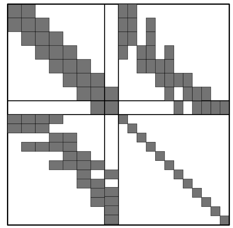
Assuming robot poses are stored sequentially, answer the following questions:

1. How many robot poses exist in this problem?
2. How many landmarks exist in the map?
3. How many landmark have been observed by the current (last) pose?
4. Which pose has observed the most number of landmark?
5. What poses have observed the 2nd landmark?
6. Predict the sparsity pattern of the information matrix after marginalizing out the 2nd feature.
7. Predict the sparsity pattern of the information matrix after marginalizing out past poses (i.e., only retaining the last pose).
8. Marginalizing out which variable (chosen among both poses or landmarks) would preserve the sparsity pattern of the information matrix?
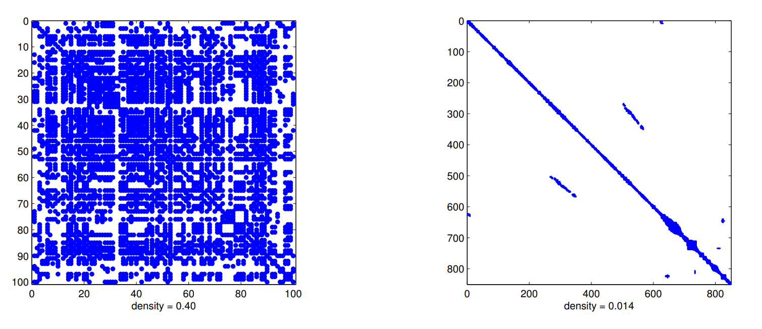
9. The following figures illustrate the robot (poses-poses) block of the information matrix obtained after marginalizing out (eliminating) all landmarks in bundle adjustment in two different datasets. What can you say about these datasets (e.g., was robot exploring a large building? Or perhaps it was surveying a small room? etc) given the spy images below?

📨 Deliverable 2 - Well-begun is Half Done [10 pts]

Pose graph optimization is a non-convex problem. Therefore, iterative solvers require a (good) initial guess to converge to the right solution. Typically, one initializes nonlinear solvers (e.g., Gauss-Newton) from the odometric estimate obtained by setting the first pose to the identity and chaining the odometric measurements in the pose graph.

Considering that chaining more relative pose measurements (either odometry or loop closures) accumulates more noise (and provides worse initialization), propose a more accurate initialization method that also sets the first pose to the identity but chains measurements in the pose graph in a more effective way. A 1-sentence description and rationale for the proposed approach suffices.

Hint: consider a graph with an arbitrary topology. Also, think about the problem as a graph, where you fix the “root” node and initialize each node by chaining the edges from the root to that node..

📨 Deliverable 3 - Feature-based methods for SLAM [10 pts]

Read the ORB-SLAM paper (available here) and answer the following questions:

1. Provide a 1 sentence description of each module used by ORB-SLAM (Fig. 1 in the paper can be a good starting point).
2. Consider the case in which the place recognition module provides an incorrect loop closure. How does ORB-SLAM check that each loop closure is correct? What happens if an incorrect loop closure is included in the pose-graph optimization module?

📨 Deliverable 4 [Optional] - Direct methods for SLAM [+5 pts]

Read the LSD-SLAM paper (available here, see also the introduction below before reading the paper) and answer the following questions:

1. Provide a 1 sentence description of each module used by LSD-SLAM and outline similarities and differences with respect to ORB-SLAM.
2. Which approach (between feature-based or direct) is expected to be more robust to changes in illumination or occlusions? Motivate your answer.

LSD-SLAM is a direct method for SLAM, as opposed to feature-based methods we have worked with previously. As you know, feature-based methods detect and match features (keypoints) in each image and then use 2-view geometry (and possibly bundle adjustment) to estimate the motion of the robot. Direct methods are different in the fact that they do not extract features, but can be easily understood using the material presented in class.

In particular, the main difference is the way the 2-view geometry is solved. In feature-based approaches one uses RANSAC and a minimal solver (e.g., the 5-point method) to infer the motion from feature correspondences. In direct methods, instead, one tries to estimate the relative pose between consecutive frames by minimizing directly the mismatch of the pixel intensities between two images:

Where the objective looks for a pose $\xi$ (between the last frame $I_{ref}$ and the current frame $I$ that minimizes the mismatch between the intensity $I_{ref}(p_i)$ at pixel $p_i$ for each pixel $p_i$ in the image, and intensity of the corresponding pixel in the current image $I$. How do we retrieve the pixel corresponding to $p_i$ in the current image $I$? In other words, what is this term?:

It seems mysterious, but it’s nothing new: this simply represents a perspective projection. More specifically, given a pixel $p_i$, if we know the corresponding depth $D_{ref}(p_i)$ we can get a 3D point that we can then project to the current camera as a function of the relative pose. The $\omega$ is typically called a warp function since it “warps” a pixel in the previous frame $I_{ref}$ into a pixel at the current frame $I$. What is the catch? Well.. the depth $D_{ref}$ is unknown in practice, so you can only optimize $E(\xi)$ if at a previous step you have some triangulation of the points in the image. In direct methods, therefore these is typically an “initialization step”: you use feature-based methods to estimate the poses of the first few frames and triangulate the corresponding points, and then you can use the optimization of $E(\xi)$ to estimate later poses. The objective function $E(\xi)$ is called the photometric error, which quantifies the difference in the pixel appearance in consecutive frames.

NOTE: LDSO (Direct Sparse Odometry with Loop Closures) which you are going to use in Part 2 of this handout is simply an evolution of LSD-SLAM (by the same authors). We are suggesting you to read the LSD-SLAM paper since it provides a simpler introduction to direct methods, while we decided to use LDSO for the experimental part since it comes with a more recent implementation.

📨 Deliverable 5 [Optional] - From landmark-based SLAM to rotation estimation [+15 pts]

Consider the following landmark-based SLAM problem:

Where the goal is to compute the poses of the robot $(t_i, R_i),\ i=1,\ldots,N$ and the positions of point-landmarks $p_k, k= 1, \ldots, M$ given odometric measurements $(\bar{t}_{ij}, \bar{R}_{ij})$ for each odometric edge $(i,j) \in \mathcal{E}_o$ (here $\mathcal{E}_o$ denotes the set of odometric edges), and landmark observations $\bar{p}_{ik}$ of landmark $k$ from pose $i$ for each observation edge $(i,k) \in \mathcal{E}_l$ (here $\mathcal{E}_l$ denotes the set of pose-landmark edges).

• Prove the following claim: “The optimization problem (1) can be rewritten as a nonlinear optimization over the rotations $R_i,\ i=1,\ldots,N$ only.” Provide an expression of the resulting rotation-only problem to support the proof.
  • Hint: i) Euclidean norm is invariant under rotations, and (ii) translations/positions variables appear …! Consider also using a compact matrix notation to rewrite the sums in the cost function otherwise it will be tough to get an expression of the rotation-only problem.
• The elimination of variables discussed at the previous point largely reduces the size of the optimization problem (from 6N+3L variables to 3N variables).However, the rotation problem is not necessarily faster to solve. Discuss what can make the rotation-only problem more computationally-demanding to solve.
  • Hint: What property makes optimization-based SLAM algorithms fast to solve?

👥 Team

Install Docker Engine

Follow the installation instructions listed here. Specifically, you should follow the instructions listed in the “Install Using the Repository” section.

Building Docker Images

We are going to build two open source SLAM approaches. The first is ORB-SLAM3, a more modern version of the system described in the ORB-SLAM paper. The second is Kimera-VIO.

First, we’ll build ORB_SLAM3:

cd /path/to/lab9
sudo docker build -f- -t orbslam:latest . < Dockerfile_ORBSLAM3

Next, we’ll build Kimera:

sudo docker build -f- -t kimera:latest . < Dockerfile_KIMERA

Prepare the Dataset

You should have the MH_01_easy sequence of the EuRoC dataset downloaded already from the last lab, but if you haven’t, download it from here and place it under the path /home/$USER/datasets/vnav/ (i.e., such that /home/$USER/datasets/vnav/MH_01_easy exists).

Running the comparison

First, you can run ORB-SLAM3 via

./run_docker.sh orbslam:latest

You should see something like this:

Wait for ORB-SLAM3 to finish running the entire sequence (it will exit automatically when finished). You should now see a file named CameraTrajectory.txt under output/orbslam.

Next, you can run Kimera via

./run_docker.sh kimera:latest

You should see something like this:

Wait for Kimera to finish running the entire sequence (it will exit automatically when finished). You should now see several files under output/kimera. We specifically care about output/kimera/traj_vio.csv.

📨 Deliverable 6 - Performance Comparison [60 pts]

Install evo, a python toolbox for evaluating the quality of trajectory estimates:

python3 -m pip install --user evo

You may find readme and wiki of evo useful.

First, we need to fix the timestamps on the ORB-SLAM3 trajectory file. Run the fix_timestamps.py script to convert the ORB-SLAM3 timestamps to nanoseconds (and to convert the Kimera-VIO trajectory to the right format).

Now you can use the evo_traj tool to plot both trajectories for MH_01_easy. Add this plot to your report and comment on the differences that you see between trajectories:

evo_traj tum output/kimera/kimera.txt output/orbslam/orb_slam3.txt --plot

In general, different SLAM systems may use different conventions for the world frame, so we have to align the trajectories in order to compare them. This amounts to solving for the optimal (in the sense of having the best fit to the ground truth) $\SE{3}$ transformation of the estimated trajectory. Fortunately, tools like evo provide implementations that do this for us, so we’re not going to ask you to implement the alignment process in this lab. Let’s compare to the ground-truth pose data from the EuRoC dataset next, taking into consideration this pose alignment.

First, convert the ground-truth trajectory for the MH_01_easy sequence to the right format:

evo_traj euroc ~/datasets/vnav/MH_01_easy/mav0/state_groundtruth_estimate0/data.csv --save_as_tum

Next, run:

evo_traj tum output/kimera/kimera.txt output/orbslam/orb_slam3.txt --ref data.tum --plot --align

Add this plot to your report and comment on the differences that you see between trajectories.

📨 [Optional] Deliverable 7 - LDSO [+10 pts]

Based on LSD-SLAM, LDSO is a direct (and sparse) formulation for SLAM. It can also handle loop closures (a limitation of the original LSD-SLAM).

Install the code for LDSO by following the Readme.md in the GitHub repository.

In the same Readme.md there is an example on how to run this pipeline for the EuRoC dataset:

cd ~/path/to/LDSO
./bin/run_dso_euroc preset=0 files=$HOME/datasets/vnav/MH_01_easy/mav0/cam0

At this point, you should be able to see the following window:

LDSO will by default output the results in results.txt in the same folder where you ran the command. You can also specify the output folder by setting the output flag when running DSO. The results file will only be generated once the sequence has been processed.

Note that the output from LDSO might be formatted incorrectly (e.g., spurious backspaces).

Plot the trajectory produced by LDSO with the trajectories from Kimera and ORB-SLAM3. Briefly comment on any differences in the trajectories.

Note that LDSO is a monocular method and there is no way of recovering the true scale of the scene. You will want to use the --correct_scale flag for evo to estimate not just the $\SE{3}$ alignment of the predicted trajectory to the ground-truth trajectory, but also the global scale factor.

Here’s an example of the aligned trajectories plotted in the x-y plane (you can add the flag --plot_mode xy to compare with this plot):

Summary of Team Deliverables

1. Comparison plots of Kimera and ORB-SLAM3 on MH_01_easy with comments on differences in trajectories
2. Plot of Kimera and ORB-SLAM3 trajectories on MH_01_easy aligned with ground-truth with comments on any differences in the trajectories
3. [Optional] Plot of Kimera + ORB-SLAM3 + LDSO (aligned and scale corrected with ground-truth) with comments on any differences in trajectories